You can read a leaderboard on a website. You cannot bend it, filter it, or chart it — and that is its own particular frustration, wanting a baseball number you can see and having no idea how to get it off the page and into your own hands. pybaseball closes that gap. It is a free, open-source Python library that pulls Major League data — season stats, Statcast pitch-by-pitch, leaderboards — straight into a pandas DataFrame, where it becomes yours to do anything with.
This is a from-scratch tutorial. By the end you will have installed the library, pulled the 2025 batting leaderboard, filtered it down to the hitters who actually played, and drawn a clean bar chart of the top ten by OPS — the exact chart below, produced by about twenty lines of code. No API key, no scraping, no spreadsheet exports. Ten minutes, start to finish.
Install it
pybaseball lives on PyPI, so installation is a single command. Open a terminal and run:
pip install pybaseballThat pulls in pandas, requests, and matplotlib as dependencies, which means you already have everything you need to fetch data and plot it. If you keep your projects in virtual environments — and you should — activate yours first. The version this tutorial was written against is 2.2.7; you can confirm what you got by running python -c "import pybaseball; print(pybaseball.__version__)". Anything in the 2.x line behaves the same way for what follows.
The imports
Three lines set the stage. We import matplotlib for plotting and pybaseball under the short alias pyb. The first line silences a thicket of harmless deprecation and SSL warnings that some of the backends emit — cosmetic, but it keeps your console readable.
import warnings; warnings.filterwarnings("ignore")
import matplotlib.pyplot as plt
import pybaseball as pyb
That is the entire setup. Everything else is two function calls and a chart.
Pull the leaderboard
Here is the single most important decision in this whole exercise, and it is one most tutorials get wrong. pybaseball can pull season batting lines from two different sources: FanGraphs (via batting_stats()) and Baseball-Reference (via batting_stats_bref()). They return similar-looking tables. They do not behave the same way for automated scripts.
FanGraphs aggressively rate-limits and frequently blocks programmatic access. Call batting_stats() a couple of times in quick succession and you will start collecting timeouts, 403s, and empty frames — not because your code is wrong, but because the server decided a robot was knocking. The Baseball-Reference and Statcast backends do not do this. They are the reliable choice, and they are what this tutorial uses throughout. So we reach for batting_stats_bref:
df = pyb.batting_stats_range("2025-03-18", "2025-09-28")
df = df[df["PA"] >= 300].copy()
top = df.sort_values("OPS", ascending=False).head(10)
Three lines, three ideas. The first hands you every 2025 player-batting line as a DataFrame — every hitter, dozens of columns, indexed and ready. Passing explicit dates matters more than it looks: those two dates are opening day and the final day of the regular season, and windowing the pull that way is what keeps October out of your season totals. Ask bref for “2025” as a whole and it happily counts postseason games too, which quietly pushes the leaders’ plate appearances past what any official leaderboard will show you. The second line filters: df["PA"] >= 300 keeps only players with at least 300 plate appearances, which throws out September call-ups and bench arms whose tiny samples would otherwise clutter the top of a rate-stat list. The .copy() is a small good habit — it tells pandas you mean to keep this slice as its own object and quietly avoids a SettingWithCopyWarning later. The third line sorts by OPS, highest first, and keeps the top ten.
Note that the column names — PA, OPS, OBP, SLG, HR — come straight from Baseball-Reference’s own headers. If you ever forget what a table offers, print(df.columns.tolist()) spells it out.
Chart the top ten
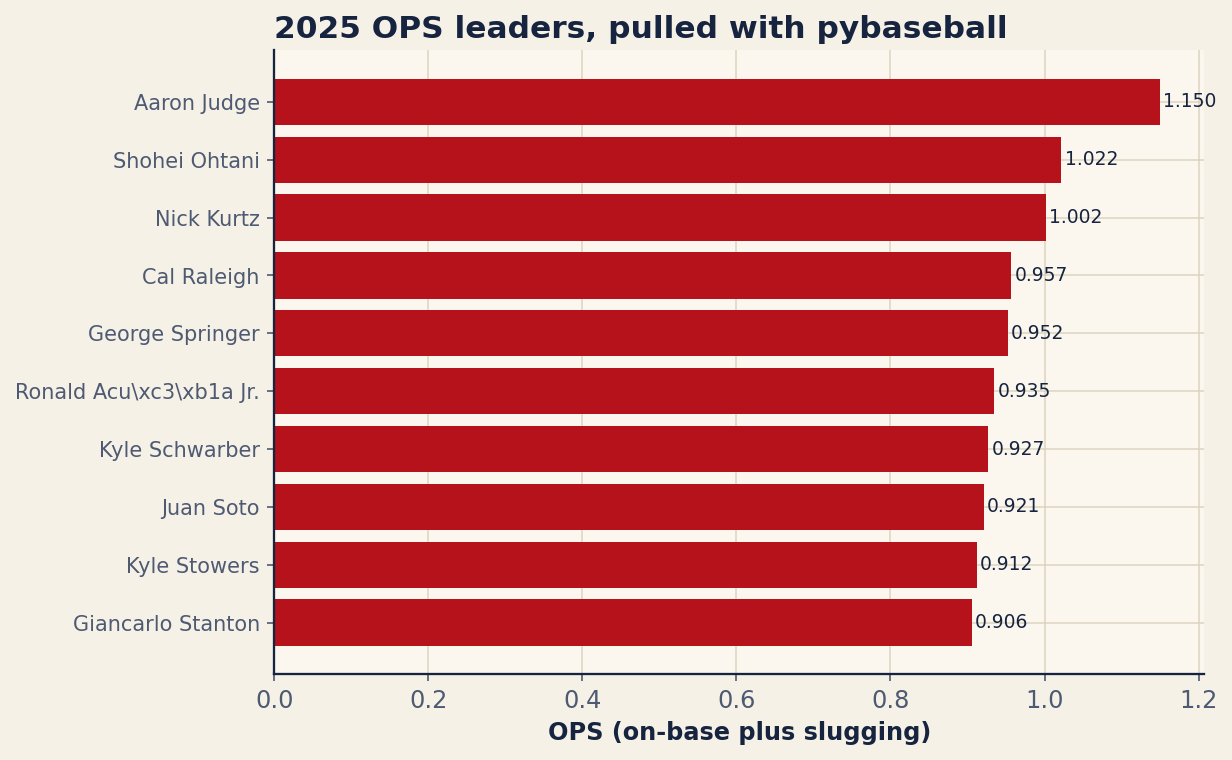
A DataFrame is useful; a picture is persuasive. We will draw a horizontal bar chart, which is the right shape for a ranked list of names because the labels read left-to-right like a leaderboard should. The setup grabs the names and OPS values out of the top frame and reverses both lists with [::-1] — matplotlib draws the first bar at the bottom, so reversing puts the best hitter on top where the eye expects him.
fig, ax = plt.subplots(figsize=(8.0, 5.4))
names = top["Name"].tolist()[::-1]
vals = [float(v) for v in top["OPS"].tolist()][::-1]

ax.barh(range(len(names)), vals)
ax.set_yticks(range(len(names)))
ax.set_yticklabels(names, fontsize=10)
ax.set_xlabel("OPS (on-base plus slugging)")
ax.set_title("2025 OPS leaders, pulled with pybaseball", loc="left")

for i, v in enumerate(vals):
    ax.text(v + .004, i, "%.3f" % v, va="center", fontsize=9)

plt.show()
The barh call draws the bars; the two set_yticks/set_yticklabels lines attach player names to them. The little for loop is the touch that makes it feel finished: it writes each OPS value as text just past the end of its bar, formatted to three decimals with "%.3f", so a reader gets both the visual length and the exact figure. Swap plt.show() for fig.savefig("ops_leaders.png") if you would rather write the chart to a file. Run the script and the figure below is what you get.
Reading what you pulled
The numbers are worth a glance, because they are a good sanity check that the pull worked. Aaron Judge sits on top at a 1.144 OPS — 53 home runs against a .457 on-base percentage and a .688 slugging mark, a line that barely looks real. Shohei Ohtani follows at 1.014, and rookie Nick Kurtz crashes the list at 1.002 on the strength of a .619 slug in under 500 plate appearances. Here is the full top ten exactly as the script saved it:
| Player | PA | HR | OBP | SLG | OPS |
|---|---|---|---|---|---|
| Aaron Judge | 679 | 53 | 0.457 | 0.688 | 1.144 |
| Shohei Ohtani | 727 | 55 | 0.392 | 0.622 | 1.014 |
| Nick Kurtz | 489 | 36 | 0.383 | 0.619 | 1.002 |
| George Springer | 586 | 32 | 0.399 | 0.56 | 0.959 |
| Cal Raleigh | 705 | 60 | 0.359 | 0.589 | 0.948 |
| Ronald Acuña Jr. | 412 | 21 | 0.417 | 0.518 | 0.935 |
| Kyle Schwarber | 724 | 56 | 0.365 | 0.563 | 0.928 |
| Juan Soto | 715 | 43 | 0.396 | 0.525 | 0.921 |
| Kyle Stowers | 457 | 25 | 0.368 | 0.544 | 0.912 |
| Will Smith | 436 | 17 | 0.404 | 0.497 | 0.901 |
That table was not typed by hand. It is the same top DataFrame, written out column by column — which is the whole point of getting data into Python in the first place. Once it is a frame, charting it, tabulating it, joining it to another season, or filtering it by team are all one line away.
Where to go next
Two functions unlock most of the rest of the library. The first is playerid_lookup, which translates a human name into the various ID numbers the data sources use:
pyb.playerid_lookup("judge", "aaron")That returns a small DataFrame with, among other columns, key_mlbam — the MLB Advanced Media ID. You need that ID for the second function, statcast_batter, which pulls a single hitter’s every tracked pitch and batted ball, complete with exit velocity, launch angle, and hit coordinates. That is the raw material for a spray chart, and it is exactly the next tutorial in this series: building a spray chart from Statcast data picks up precisely where this one leaves off, turning statcast_batter output into a picture of where a hitter sprays the ball.
A short troubleshooting note
Three things trip up newcomers. First, rate limits: if a call hangs or returns nothing, you are almost certainly hitting a FanGraphs endpoint — switch to the Baseball-Reference or Statcast equivalents, and do not hammer any source in a tight loop. Second, caching: pybaseball can remember responses so you are not re-downloading the same data on every run, which is both faster and friendlier to the servers. Enable it once with from pybaseball import cache; cache.enable() and repeated pulls come back instantly. Third, an empty DataFrame usually means a season hasn’t started or a name was misspelled, not that anything is broken — check your arguments before you check your code.
The bottom line
The distance between “I wish I could chart that” and an actual chart is, it turns out, about twenty lines of Python and one good decision about which backend to trust. Install pybaseball, lean on the Baseball-Reference and Statcast sources, get your data into a DataFrame, and the entire toolbox of pandas and matplotlib opens up behind it. You now have the leaderboard in your hands — bend it however you like.
Sources & Further Reading
- Background reading: Chapter 7: Introduction to pandas, a free textbook chapter at DataField.dev.
- Leaderboard data: Baseball-Reference, pulled via pybaseball’s Baseball-Reference daily backend (version 2.2.7), windowed to the 2025 regular season (March 18 – September 28; postseason excluded). Numbers retrieved July 2026; re-runnable via
scripts/pybaseball_quickstart.py. - Baseball Savant — the Statcast source behind
statcast_batterand the spray-chart follow-up. - FanGraphs — an alternate stats backend, noted here for the rate-limiting caveat discussed above.