Half of run differential lives in one file and half lives in another, and the entire skill of this tutorial is getting them into the same row. Runs scored is a batting stat; runs allowed is a pitching stat; the sources that publish them almost never publish them together. So the single most common real task in baseball analysis isn’t a fancy model — it’s a join: matching two tables on a shared key so you can do arithmetic across them. Do that once here, on real 2024 data, and you’ll have built a run-differential and Pythagorean table for all 30 teams from parts that started out apart.
The plan: load two bundled JSON files — team batting and team pitching — join them on team_id, compute each team’s run differential and Pythagorean expected wins, sort the result, and find the luckiest team in baseball. No pandas required; the standard library does all of it. But we’ll show the pandas version too, because a join is where pandas actually earns its weight.
Why the join is the whole problem
Run differential is trivial arithmetic — runs scored minus runs allowed — and it’s the sturdiest one-number summary of team quality there is, correlating with wins far more tightly than any single side of the ball. The catch is purely logistical. Our batting file lists each team’s runs (scored) with a short name like "Padres". Our pitching file lists each team’s runs_allowed with a full name like "San Diego Padres". If you tried to match them on the team name, you’d fail on all 30, because the strings don’t agree.
This is exactly why you join on an ID, not a label. Both files carry a stable team_id — the same integer the MLB Stats API uses for a franchise regardless of how it spells the name. Match on that and the naming mismatch evaporates. The lesson generalizes: whenever you merge two baseball datasets, hunt for the numeric key first and treat the display name as decoration.
Step 1: load the two files
Both datasets ship in the site’s data_layer/ folder as JSON, each a dictionary with a "teams" list. Loading them is three lines with the standard library:
import json

with open("data_layer/team_batting_2024.json", encoding="utf-8") as f:
    batting = json.load(f)["teams"]
with open("data_layer/team_pitching_2024.json", encoding="utf-8") as f:
    pitching = json.load(f)["teams"]

print(len(batting), len(pitching))   # 30 30
Each element of batting looks like {"team": "Padres", "team_id": 135, "runs": 760, "W": 93, ...} and each element of pitching like {"team": "San Diego Padres", "team_id": 135, "runs_allowed": 669, "W": 93, ...}. Different names, same team_id. That shared integer is our hinge.
Step 2: the join
The pattern for joining without pandas is to turn one table into a lookup keyed by the join column, then walk the other table and pull the matching partner. A dictionary comprehension builds the index in one line:
# index pitching by team_id for O(1) lookup
pitch_by_id = {t["team_id"]: t for t in pitching}

rows = []
for b in batting:
    p = pitch_by_id.get(b["team_id"])
    if p is None:
        continue                       # no match: skip rather than crash
    rows.append({
        "team": b["team"],
        "RS":   b["runs"],             # runs scored, from batting
        "RA":   p["runs_allowed"],     # runs allowed, from pitching
        "W":    b["W"],
    })

print(len(rows))                       # 30 — every team matched
That .get() with a None check is not decoration — it’s the honest way to handle a key that might not match. If a team existed in one file but not the other, this skips it instead of raising a KeyError, and the len(rows) check tells you whether every team found its partner. Here all 30 do. Now each row holds runs scored and runs allowed together, which is the thing neither file had on its own.
Step 3: run differential and Pythagorean wins
With both numbers in the same row, the arithmetic is immediate. Run differential is a subtraction. Pythagorean expected wins — Bill James’s estimate of the record a team’s run scoring and prevention “deserved” — uses the runs-squared form, here with the widely used 1.83 exponent instead of James’s original 2:
for r in rows:
    r["diff"] = r["RS"] - r["RA"]
    exp = r["RS"]**1.83 / (r["RS"]**1.83 + r["RA"]**1.83)
    r["pyW"] = round(exp * 162, 1)     # expected wins over a 162-game season
    r["luck"] = round(r["W"] - r["pyW"], 1)   # actual minus expected

rows.sort(key=lambda r: r["diff"], reverse=True)
The luck column — actual wins minus Pythagorean wins — is the interesting one. A positive value means a team won more games than its run differential suggested it should have, usually by going better than expected in one-run games; a negative value means it left wins on the table. It’s the residual the whole Pythagorean model is built to expose.
The result: 2024, joined and ranked
Print the sorted rows and you get the table below — the top and bottom of the league by run differential, assembled entirely from two files that never shared a row until we joined them:
| Team | RS | RA | Diff | Actual W | Pyth W | Luck |
|---|---|---|---|---|---|---|
| Dodgers | 842 | 686 | +156 | 98 | 96.0 | +2.0 |
| Yankees | 815 | 668 | +147 | 94 | 95.6 | −1.6 |
| Brewers | 777 | 641 | +136 | 93 | 95.1 | −2.1 |
| Phillies | 784 | 671 | +113 | 95 | 92.5 | +2.5 |
| D-backs | 886 | 788 | +98 | 89 | 89.7 | −0.7 |
| … 20 teams omitted … | ||||||
| Angels | 635 | 797 | −162 | 63 | 64.4 | −1.4 |
| Marlins | 637 | 841 | −204 | 62 | 60.8 | +1.2 |
| Rockies | 682 | 929 | −247 | 61 | 58.7 | +2.3 |
| White Sox | 507 | 813 | −306 | 41 | 48.0 | −7.0 |
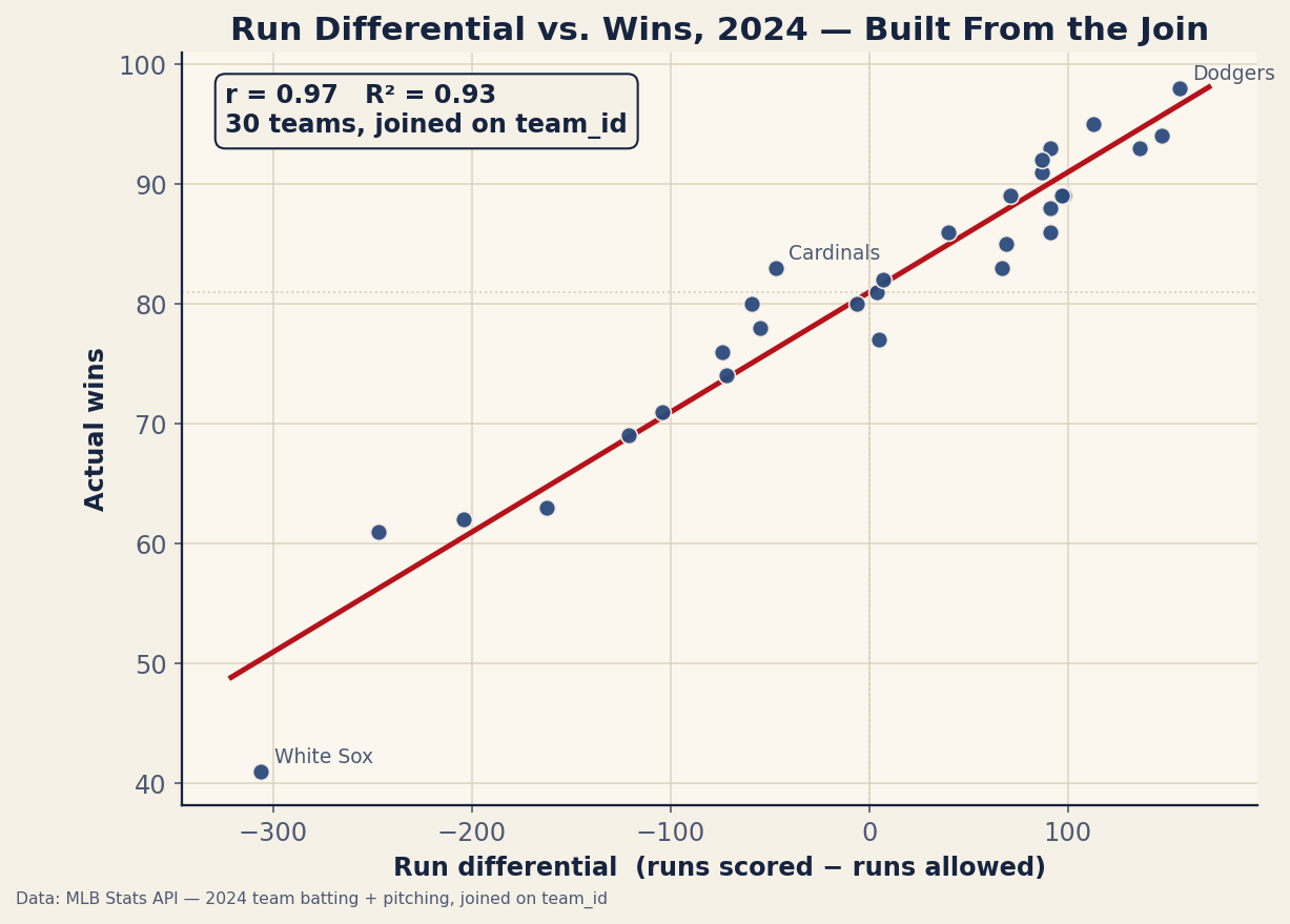
A couple of real findings fall right out of the joined table. Run differential tracks actual wins across the 30 teams at r = 0.97 — the reason it’s the backbone of any power ranking. And the luck column names the extremes: the 2024 Cardinals were the luckiest team in baseball at +7.0 wins (a −47 differential that somehow produced 83 wins), while the White Sox were the unluckiest at −7.0 — their historically bad 41-win season was, astonishingly, a few games worse than even a −306 differential predicted. Neither of those facts is visible in either source file alone. The join is what surfaced them.
The pandas version
The standard-library approach is worth understanding because it shows you what a join actually is — an index and a lookup. But once you trust the concept, pandas does the same work in fewer lines and handles the bookkeeping for you:
import pandas as pd, json

bat = pd.DataFrame(json.load(open("data_layer/team_batting_2024.json"))["teams"])
pit = pd.DataFrame(json.load(open("data_layer/team_pitching_2024.json"))["teams"])

df = bat.merge(pit[["team_id", "runs_allowed"]], on="team_id")   # the join
df["diff"] = df["runs"] - df["runs_allowed"]
exp = df["runs"]**1.83 / (df["runs"]**1.83 + df["runs_allowed"]**1.83)
df["pyW"] = (exp * 162).round(1)
df["luck"] = (df["W"] - df["pyW"]).round(1)

print(df.sort_values("diff", ascending=False)
        [["team", "runs", "runs_allowed", "diff", "W", "pyW", "luck"]])
The one line that matters is bat.merge(pit[...], on="team_id"). That’s the same join, declared instead of hand-rolled: match rows where team_id agrees, and glue the columns together. We selected only team_id and runs_allowed from the pitching frame on purpose — both files also carry W and team, and merging them whole would leave you with awkward W_x/W_y duplicate columns. Pulling just the column you need from the right-hand table is the small habit that keeps a merge clean.
Where this can bite you
- Mismatched keys silently drop rows. A default pandas
mergeis an inner join — teams present in only one frame vanish from the result with no warning. Always check that your row count survived the merge (len(df) == 30), exactly as the.get()-and-skip pattern made explicit above. - Never join on names. This whole tutorial exists because the two files spell team names differently. Franchise relocations, nicknames, and accents make string joins fragile; the numeric
team_idis the stable key. Reach for it every time it exists. - The exponent is a choice. We used 1.83; James’s original was 2, and a season-fit value can differ — it barely moves the standings, as our piece on fitting the Pythagorean exponent shows, but be explicit about which you used.
- Luck is a residual, not a verdict. A +7 “lucky” team isn’t proven lucky; the gap also absorbs bullpen quality and one-run-game skill. It’s a flag for a closer look, which is the spirit of our runs-per-win work.
If you’d rather skip the code and just feel how runs scored and allowed become an expected record, the site’s Pythagorean calculator does it live:
Interactive tool
Pythagorean Win Expectation
Expected winning percentage and a projected W–L record from runs scored and runs allowed. This interactive calculator needs JavaScript. The formula it uses is printed on this page, so the method works without it.
The bottom line
Run differential looks like a single stat, but building it for every team is really a data-wrangling exercise: two files, one shared team_id, one join. Index the second table by the key, look up each row’s partner, and suddenly runs scored and runs allowed sit side by side, ready for a subtraction and a Pythagorean estimate. The payoff is findings neither source file held alone — that 2024 differential tracked wins at r = 0.97, and that the Cardinals (+7) and White Sox (−7) were the season’s luck extremes. Learn the join on this small, clean example and you’ve learned the move that most real baseball analysis is quietly made of.
Sources & Further Reading
- 2024 team batting and pitching: bundled
data_layer/team_batting_2024.jsonanddata_layer/team_pitching_2024.json, pulled from the MLB Stats API (retrieved 2026-06-22 and 2026-06-24). - pandas
mergedocumentation — join types (inner/left/outer) and how key matching works. - Bill James — the Pythagorean win expectation, introduced in the Baseball Abstract; background via SABR.
- Related: Build a run-differential power ranking and what Pythagorean exponent fits best — where this joined table leads next.